 Using Fourier analysis to identify the most significant subdivisions of a centuriation |
In certain parts of the Salentine cadastre, which is a typical centuriation with a module of 705m, there are also many other existing boundaries at the same orientation as the grid, which may be the remains of regular limites intercisiui. Compatangelo looked for signs of subdivision because this may give clues to this cadastre's date and function, by allowing comparison with other better known Roman cadastres.
Her approach was to generate periodograms - charts which show the relative importance of frequencies contributing to the observed pattern. Frequencies with large amplitude may reveal underlying regularities in the field pattern, even in the presence of "noise" arising from later modifications.
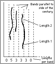 Periodograms are obtained by generating Fourier transforms of n values which represent the distribution of the data within some fundamental interval. In this case the numbers are derived from a figure proportional to the length of boundaries falling in a series of n equally spaced bands parallel to one orientation of the cadastral grid (see figure, left). In order to compensate for degradation of the traces, which may have become irregular or been wiped out, data is summed from the corresponding bands of several grid squares. Thus the fundamental interval is the module of the centuriation, and within this interval we have n values forming a real vector z.
The Fast Fourier transform (FFT) takes this vector z and creates a vector c whose values are the complex coefficients of of the discrete Fourier transform of z. In the case of the MathCAD FFT routine used by the author, these coefficients satisfy
FFT routines will produce (n/2)+1 values of c, and the periodogram is the set of absolute values of c. The periodogram values are proportional to the amplitudes of cosine curves (with different phases) which, when added together, generate the distribution represented by the vector z. The periodogram values thus show the relative importance of the frequencies, and the corresponding phases measure the degree to which the cosine wave at that frequency is "in step" with the fundamental interval. It is important to take account of the phase, since only a cosine curve with phase zero close to zero will have maxima near the ends of the fundamental interval, and will thus represent a true subdivision at that frequency.
Compatangelo's raw data took the form of possible limites intercisiui summed over 20 squares. She divided the fundamental interval of 705m into 44 bands and produced three measures for each band: the sum of the length of traces, the number of occurrences of a trace and the ratio of these two. The periodograms of these discrete distributions have peaks which may represent the sought-for original divisions. For example, one of her figures (Compatangelo 1989: fig 53) shows highest amplitudes at frequencies of 2, 6, and 20, and possibly at 7 and 11. She appears to consider all of these to be potentially meaningful.
I have simulated the distribution of traces that we would expect to see in a regularly divided cadastre (Peterson 1992). Two examples of misleading output were obtained.
The corresponding values for each east-west row of grid squares were then summed (in the north-south direction) to give an array of 1024 values representing the east-west distribution of the boundaries. Then the corresponding values in each of the 16 blocks of 64 cells in this array were summed to obtain the sum of all the data. The periodogram of this distribution has a high peak, of 3.1 times the mean amplitude, at frequency 1 and a next highest peak, of just over twice the mean, at frequency 3.
But what is the statistical significance of these peaks? How often would peaks this high be obtained by chance? In order to answer this question a new array of 1024 values was constructed by assigning, to each cell, a value taken from a randomly determined cell in the original array of 1024 values. This data set was then reduced to 64 values by the procedure described above. The aim was to produce a data set with approximately the same mean and variance as the original, but in which any sign of periodicity would have been destroyed.
This randomisation process was repeated 100 times and the 3,200 periodogram values were calculated. This showed that none of the randomly generated values exceeded three times the mean value, but 4% are higher than twice the mean value. At first glance 4% looks quite a low chance; but, given 32 values in each periodogram, it is likely that at least one will exceed this level. If we use the value of 4%, then the probability is 1 - 0.9632 i.e. 0.73.
Nevertheless, one might think that the chance that two values exceed twice the mean value would be considerably lower. But, again using the 4% figure, we can calculate that the chance of seeing exactly one value exceeding twice the mean value is 0.36. Thus the probability of seeing a periodogram with at least 2 such values is 0.73 - 0.36 = 0.37. Hence, in terms of the significance of particular frequencies, the periodogram obtained in this case is not at all unusual and, furthermore, one prominent frequency could be a harmonic of the other.
However, when I looked at the phases I felt I could be a little more positive. The component with frequency 1 is out of phase by 56°, whereas that with frequency 3 is out of phase by 22°. Thus I could calculate the absolute displacement of the positions of the maxima of the respective Cosine curves from their "in phase" positions (the positions in which they coincide with the limits of the fundamental interval).
The component with frequency 1 has wavelength 709.5m; thus a phase of 56° represents a spatial displacement of the Cosine curve from the "in phase" position, of 111m. This is large. The wavelength of the component with frequency 3 is 709.5/3 = 236.5m and its phase is 22°. Thus its spatial displacement is 15m. Hence this component is much more nearly in phase, which suggests that it is unlikely to be solely a harmonic of the component with frequency 1, because there is 96m between their maxima. Despite the lack of statistical significance of its amplitude, it may indicate a genuine original subdivision of the cadastral squares into three.
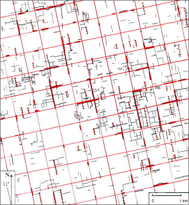
Using this clue we can select those supposed physical traces which would correspond to this form of division (dotted lines in the figure above) thus confirming the suggestion made by the Fourier analysis, that a division into 3 is present.
It is worth noting that the other relatively high values in the periodogram had even less statistical significance, nor did they appear to derive from a form of subdivision which was visible on the ground.
(e-mail j.peterson@uea.ac.uk)