

 |
||||||
UM Matlab visualisation code
This webpage contains the Matlab code I have written for basic visualisation of limited area model output from the UM 6.1. Thanks to Jeff Chagnon, Stephen Outten and Nina Petersen for help. The code may be updated from time to time. If you have any interesting comments, then please get in touch. The code works for the UK "test" simulation, job xcbmh, available via the UMUI at Reading. Note, much of it is STASH-dependent. Do not expect to use this code without making personal adjustments. Have fun!
Code |
Description |
Comments |
| um2nc.tcl | convsh/xconv script that converts a UM output file (*.pp) to a netCDF (*.nc) file. It also interpolates the C-grid variables (u,v,taux,tauy, pv, etc) onto the A-grid. | Note the interpolation requires the A-grid details: take these from the UMUI (not xconv); and the variable list number for each variable (use xconv to find these numbers). Written by Nina Petersen. |
| um_read_nc.m | Reads a netCDF file. Inputs: file location, UM pole lat and lon.
Input variable names are STASH dependent, so will need checked. Output variable names are defined here.
Variables are generally called "q" for 4D variable, or "q_sfc" at a specified level. Field values are stored as 4D arrays; e.g. q(time, levels, y, x). Calls um_xy_nc.m. |
Uses the standard Matlab netCDF toolbox. Also uses snctools nc_dump (but this could be commented out). Written by Ian Renfrew Aug 2006; based on read_nc by Jeff Chagnon, 2006 |
| um_xy_nc.m | Calculates real latitude and lontitude variables for the UM, given the UM (equatorial) coordinates. Input: (x,y); Output (x_p, y_p), where lat = y_p(i,j); lon = x_p(i,j) |
Based on UM code eqtoll.F; see the "Joy of the New Dynamics" eqns (2.27)-(2.29). Code written by Jeff Chagnon. |
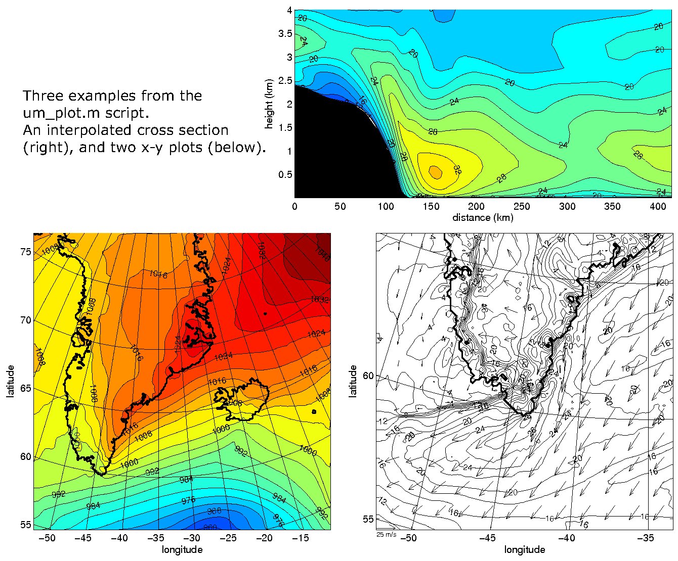
| um_plot.m | Basic plotting program on model domain. |
There is a check that overplotted fields are at the same time as the primary field. Written by Ian Renfrew, Aug 2006. Modified by Guðrún Nina Petersen and Stephen Outten. Based on code provide by Jeff Chagnon. |
| um_set_field.m | Sets details of the field to be plotted, called for each variable from um_plot. Sets variables: plotfield, fieldname and dim1, dim2 (the field dimensions; matrices); plus vtype (vertical coordinate type: Mrho, Mtheta, theta, pressure or single level) and conlevs (the contour levels). Also calculates interpolation for height-distancecross sections. |
Written by Ian Renfrew, Aug 2006. Modified by Stephen Outten |
| um_add_vectors.m | Adds velocity vectors to a plot. Vectors set via ivar_vec in um_plot. Basic command is quiver(dim2, dim1, vec1, vec2). |
Problem: this currently uses zonal & meridional winds, when really grid-relative dx/dt & dy/dt winds are more appropriate. Bug: I can only get the scaling arrow to plot within the plotting domain. Also it can be overplotted by the orography in x-z plots. Written by Ian Renfrew, Aug 2006. |
| um_level_test.m | Checks if level asked for in um_plot.m is available | Written by Guðrún Nina Petersen. |
| um_time_test.m | Checks if time asked for in um_plot.m is available |
Written by Guðrún Nina Petersen. |
| um_ancil_netcdf_sst.m | Saves variables from Matlab to a netcdf, ready to be converted to a UM ancillary file using xancil. Code must be adjusted for each ancillary file. Currently setup to create a SST ancillary file. |
Written by Guðrún Nina Petersen. |